While the ideas of gravity and acceleration at and above Earth's surface
are taught in first year physics, the acceleration due to gravity below the
surface is often ignored or approximated with a homogeneous Earth.
This essay describes a method of finding the gravitational acceleration
within a spherical approximation of Earth using a variable density function.
The gravitational acceleration at some distance away from a
point mass is given by

where
|
|
|
|
| ag |
= |
Acceleration towards mass M, m·s-2 |
| G |
= |
6.6743×10⁻¹¹ m3·kg-1·s-2 |
Universal gravitational constant 1 |
| M |
= |
Mass, kg |
| r |
= |
Distance from the center of mass, m |
The acceleration due to gravity external to a spherically symmetric
uniform and continuous distribution of mass can be described by the same equation.
Thus, if we make the assumption that the Earth is a sphere, we can
use this equation to find the acceleration due to Earth's gravity for any
position on or above the Earth's surface.
But what of the acceleration below the surface?
For a
spherically symmetric uniform and continuous distribution of mass, the mass closer to the center of the
distribution than the position in question provides a net gravitational acceleration at that position.
The acceleration produced by the shell of mass further from the center,
however, sums to zero. A good
tutorial on that fact may be found here.
If we make the assumption that the Earth's density is
constant with radius—i.e., that the Earth is homogeneous—then the acceleration
falls off in a linear fashion, reaching zero at the center. That is,
if a distribution of mass is spherically symmetric and homogeneous, we could
simply calculate the volume of a sphere at radius r and multiply that volume
by the density to find the mass. Since acceleration is proportional to
1/r2 while volume (and hence mass) is proportional to r3, then acceleration is proportional to r
within a solid sphere of constant density.
While we will assume that the Earth is spherically symmetric, it is most
certainly not homogeneous. The Earth's density is anything but constant
with respect to radius, ranging from 13,000
kg·m-3 at the center to 1,000 kg·m-3 at the surface.
There are large discontinuities in density between the various material
layers within the Earth. Moreover, within each material layer the density
can change in a non-linear fashion.
What we need is a function that will provide the mass contained in a sphere
of a given radius that allows the density to change with respect to that
radius. If we can calculate the mass, then we can calculate the
acceleration due to gravity for that mass.
The solution is to characterize each layer's density as a
function of radius, then integrate the density of each layer over radius to
find mass. Since we're assuming the Earth to be spherically symmetric,
it'll then be easy to calculate the acceleration due to gravity for any
point within the Earth.
The Preliminary Earth Reference Model (PREM) 2 provides
a table of densities at different radii within the Earth. A spreadsheet can
be used to generate a quadratic density function to fit the data points for each
material layer. The
Excel spreadsheet I used may be found here.
We end up with the following piecewise function for the Earth's density
where r is the distance from the center of the Earth and where
and
where the indexed constants for each piece of the function are described in
the table below.
|
| i |
Layer |
Height hi (m) |
ai (kg·m-5) |
bi (kg·m-4) |
ci (kg·m-3) |
| 1 |
Inner core |
1.2215×10⁶ |
-2.1773×10⁻¹⁰ |
1.9110×10⁻⁸ |
1.3088×10⁴ |
| 2 |
Outer core |
3.4800×10⁶ |
-2.4123×10⁻¹⁰ |
1.3976×10⁻⁴ |
1.2346×10⁴ |
| 3 |
D'' layer |
3.6300×10⁶ |
0 |
-5.0007×10⁻⁴ |
7.3067×10³ |
| 4 |
Lower Mantle |
5.7010×10⁶ |
-3.0922×10⁻¹¹ |
-2.4441×10⁻⁴ |
6.7823×10³ |
| 5 |
Inner transition zone 1 |
5.7710×10⁶ |
0 |
-2.3286×10⁻⁴ |
5.3197×10³ |
| 6 |
Inner transition zone 2 |
5.9710×10⁶ |
0 |
-1.2603×10⁻³ |
1.1249×10⁴ |
| 7 |
Outer transition zone |
6.1510×10⁶ |
0 |
-5.9706×10⁻⁴ |
7.1083×10³ |
| 8 |
Low velocity zone & lid |
6.3466×10⁶ |
0 |
1.0869×10⁻⁴ |
2.6910×10³ |
| 9 |
Inner crust |
6.3560×10⁶ |
0 |
0 |
2.9000×10³ |
| 10 |
Outer crust |
6.3680×10⁶ |
0 |
0 |
2.6000×10³ |
| 11 |
Ocean |
6.3710×10⁶ |
0 |
0 |
1.0200×10³ |
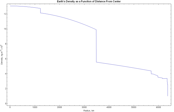
If we plot this function over the radius of the Earth, we obtain the
following.
Click on the plot thumbnail for a high resolution image
best viewed with a 1280x1024 screen resolution.
The Mathematica source code may be found here.
We can find the mass within a sphere of any radius h by
integrating the density function ρ(r) in spherical coordinates.
If the Earth's density were not a piecewise function, this would be straightforward
integration. However, since the density function contains inconvenient discontinuities,
we have to integrate each piece of the function—i.e.,
each material layer—separately, then sum the masses of each
layer appropriately.
As an example, let's derive the equation for the mass of the outer core
"below" a height h that lies somewhere within the outer
core. Note that we only want the portion of the outer core's mass
below h, but we do not want to include the mass of the inner core
since it falls under a different piece of the density function.
We start by setting up the integral of the density function for i = 2
with limits from h1 to h. Note that h is a variable while h1 is the height of
the inner core to outer core boundary given in the table above.
where the values of the indexed constants come from the density function
table shown above.
The mass functions for the other layers may be similarly derived—but
it's fairly obvious that the only difference will be in the indexed
constants.
The mass of the entire ith layer is therefore
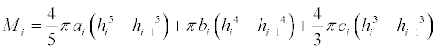
where the values of the indexed constants come from the density function
table shown above.
To calculate the total mass "below" a given radius r, we sum the
masses of the layers that are completely "below" height r, then add the partial
mass of the layer that contains radius r. In the equation
below, the height of radius r lies within the nth layer.

where the values of the indexed constants come from the density function
table shown above.
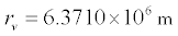
Using the volumetric radius of the Earth, 6.3710×10⁶ m, this
function evaluates to a total Earth mass of 5.9727×1024 kg.
This is only 0.015% lower than the NASA figure of 5.9736×1024 kg. 3 That's very close given that the PREM densities
were inferred from the speed of sound within the Earth using seismographic
data.
If we wish to approximate the Earth's internal structure using a constant, average density, we
can simply use the volume of a sphere with radius r.
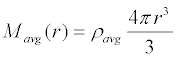
which is what that triple integral reduces to when the integrand is a
constant, and where
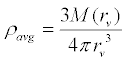
and where rv is the volumetric radius of the Earth.
The average density of the Earth evaluates to 5.5139×10³ kg·m-3.
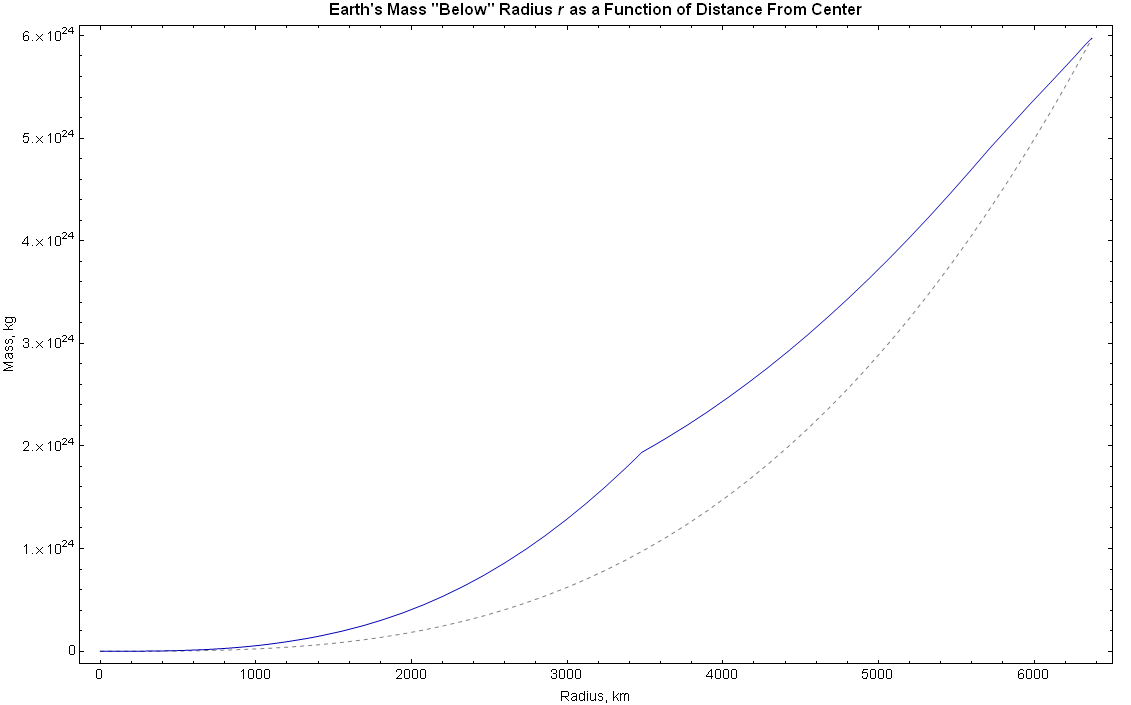
Plotting the functions for mass over the radius of the Earth, we obtain the
following. The blue line represents the true mass profile, while the dashed
gray line represents the average density approximation.
Click on the plot thumbnail for a high resolution image
best viewed with a 1280x1024 screen resolution.
The Mathematica source code may be found here.

Now that we have a fairly accurate picture of the mass distribution within
the Earth, we can return to where we started; that is, to deriving a function for the
acceleration due to Earth's gravity that works as well below the surface as
it does above.
As discussed above, the gravitational acceleration at some distance away from a
point mass or spherically symmetric distribution of mass is given by
where
|
|
|
|
| ag |
= |
Acceleration towards mass M, m·s-2 |
| G |
= |
6.6743×10⁻¹¹ m3·kg-1·s-2 |
Universal gravitational constant 1 |
| M |
= |
Mass, kg |
| r |
= |
Distance from the center of mass, m |
To account for a variable mass and variable density, we substitute our function for mass into the equation for gravitational
acceleration. We also provide a condition for radii outside the Earth.
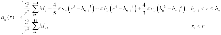
where the values of the indexed constants come from the density function
table shown above.
In the same fashion, we can also generate a function using the average
density..
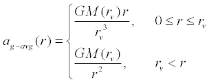
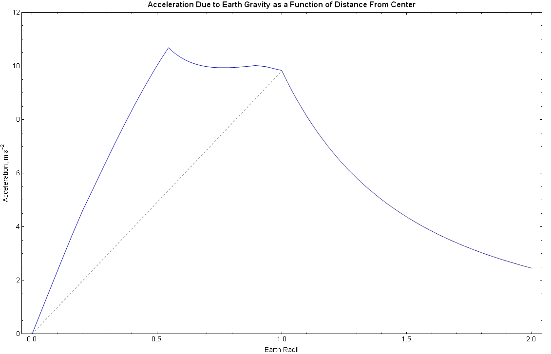
Plotting our function for the radius of the Earth, we obtain the
following. The blue line represents the true gravitational acceleration
profile, while the dashed gray line represents the gravitational
acceleration using the average density approximation.
Click on the plot thumbnail for a high resolution image
best viewed with a 1280x1024 screen resolution.
The Mathematica source code may be found here.
The value calculated for gravitational acceleration at Earth's volumetric
radius is 9.8212 m·s-2.
According to the World Geodetic System 1984 (WGS84), the true surface
acceleration on Earth varies from 9.7803 m·s-2 on the equator to
9.8322 m·s-2 at 90° latitude;
the mean value is 9.7976 m·s-2. 4 Thus, our
derivation is higher than the mean by 0.24%. A slight disagreement
with true surface acceleration is to be expected since our derivation does
not account for centripetal acceleration or the fact that the Earth is an
oblate spheroid, not a
sphere. Both phenomena are caused by the
Earth's rotation.
For reference, the WGS84 gravity formula, which takes these phenomena into account, is: 4
where
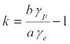
where
|
|
|
|
| γ(f) |
= |
Net surface acceleration,
m·s-2 |
| f |
= |
Geodetic latitude (map latitude) |
| γe |
= |
9.7803253359
m·s-2 |
Surface acceleration at the equator |
| γp |
= |
9.8321849378
m·s-2 |
Surface acceleration at the poles |
| a |
= |
6378137.0 m |
Semi-major axis of the Earth ellipsoid |
| b |
= |
6356752.3142 m |
Semi-minor axis of the Earth ellipsoid |
| e |
= |
8.1819190842622×10⁻² |
First eccentricity of the Earth ellipsoid |
References
1 NIST - CODATA Value: Newtonian constant of gravitation.
2 Preliminary Reference Earth Model (PREM) (Dziewonski & Anderson, 1981).
3 NASA/GSFC -
Planetary Fact Sheets.
4 DOD World Geodetic System 1984, 3rd edn., Amendment 1, Jan. 2000.
|